
5 - The Spin Quantum Number

Abstract (TL;DR):
The Spin Quantum Number begins with an experiment by Otto Stern and Walther Gerlach, which demonstrated a beam of atoms that were split evenly into two. This is due to a property of the electrons wherein they generate their own internal momentum. This momentum, called a “spin,” determines this final quantum number.
—
Originally posted by geometricanimations
Updated 4/2026.
This is it! We have finally reached the conclusion of orbitals. I can already hear the cheers from the Chemistry 101 students reading this. Let’s march on and finish up.
Be sure to check out Part 4 before this one. You can’t understand where this one begins without seeing where the other one ends.
Now, it is time to explain the last quantum number.
The Quantum Dive - Internal Energy
Stern-Gerlach Experiment
Electrons are trying to get rid of their energy in any way possible. Orienting themselves in a way that lowers energy is a good starting point, but they still have plenty of internal energy. In fact, electrons have their own internal angular momentum, separate from the orbital angular momentum (l).

The Stern-Gerlach Experiment Setup
(1) The emitter for the silver atom beam. (2) The silver atom beam. (3) The nonuniform magnets (north and south poles are different shapes, distorting the magnetic field). (4) What they expected the result to be. (5) What the result actually was.
This was determined after a 1921 (and follow-up 1922) experiment by German physicist Otto Stern and Walther Gerlach. The aptly named Stern-Gerlach Experiment sought to identify if electrons were truly following the quantum mechanical rules that the path of Bohr set us on. This experiment would ultimately assist Louis de Broglie in identifying the dual-nature of electrons that we covered in Part 2.
The setup involved firing a beam of silver atoms through a nonuniform magnetic field and observing the results on a detecting wall at the end. The result, surprisingly, was that the beam was deflected in only two directions, landing flush against the detector in exactly two spots.
But how could that be? If you think about it, if you threw twenty bar magnets at a magnetic wall past two huge magnets and looked at where they ended up, they would all be stuck on the wall in random places. After all, you have no idea what direction those magnets were when you threw them or how much attraction or repulsion one magnet had than another one, so you should have no idea exactly how they will come out. Shouldn’t it have been the same for these atoms?
In order to explain the significance of this inconsistency, I’ll need to diverge for a second into the physical quantity of momentum.
Types of Momentum
We’ve spent quite a bit of time talking through orbital angular momentum. But there are several types. First, of course, is linear momentum, the momentum all physics students are likely familiar with. This momentum is acquired by multiplying a mass by its velocity, or its displacement over some time in some direction. This tells you how much, in numerical form, an object moves in a particular direction. In fact, you likely already knew the definition of “momentum” without knowing how to put it in words. Classical angular momentum is almost completely the same. The only difference is that an axis is involved, around which your mass rotates.
For classical angular momentum, instead “mass” and “velocity,” the two relative quantities are the rotational inertia (also known as the moment of inertia or angular mass) and angular velocity. The latter is simply the rate at which rotation occurs about some axis. On the other hand, the rotational inertia, is used to depict how much torque, or rotational force, you need to move an object a certain distance around an axis with respect to a certain position. The classic example of this is the tightrope walker.

If it was super easy to make an acrobat flip around the rope (for example, if gravity didn’t exist), then you would say that their moment of inertia is low. But when one walks across a rope you usually see them stick their arms out or hold a long rod. That single act increases the moment of inertia because you have changed the center of the mass, where the force acts. That is, more rotational force would be needed to rotate the acrobat.
With this foundation in momentum, we have one tool to explain the final quantum number.
Magnetism
The next tool comes through an explanation of the electron’s behavior and its innate properties.
First, before I discuss their behavior, we need to review a few things about electrons. Electrons are not individual points or balls of negative charge. They’re objects with wave-like and particle-like qualities (that we call and treat as particles for the sake of discussion or math). Its location at any given moment is best shown with a cloud of probabilities (the electron cloud model shown back in Part 1). This is why we call the patterns of their motion “orbitals”, which represent that cloud, and not “orbits”.
With that in mind, I mentioned in Part 2 that electrons, as charged particles, can generate a magnetic field just by moving. We also know that electrons are “moving” around the nucleus, and, therefore, they must be exhibiting some sort of magnetic field.
This is known as orbital magnetization, which causes the electron to behave like magnetic dipoles, which are objects with two opposing poles that generate magnetic fields (like a bar magnet or the north and south pole of the Earth). If the electrons had become magnetic dipoles in this way, then, when the silver atoms passed through the magnets that Stern and Gerlach set up, they would have been influenced by the attractive and repulsive magnetic forces (like poles repel, opposite poles attract). More specifically, depending on the orientation of the electrons in the silver atoms, they would land on the opposing detector nearer to one of the two magnets or somewhere in between (hence the prediction of a line pattern).
Crucially though, the creation of this kind of magnetic field requires circulation around a nucleus, like a loop. If there is no net movement around the nucleus, there wouldn’t be any kind of magnetic field created from the electron’s movement. There is one such orbital that fits this situation, and, believe it or not, you’ve already read about it - the “s” orbital.
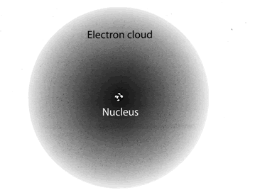
This is a representation of the 1s orbital in electron cloud form. The cloud looks grainy, right? Each of those grains is a possible location for an electron.
In Part 4, we explained that the “s” orbital corresponds to an orbital quantum number (l) of 0, which means the electron itself has an orbital angular momentum of 0. From our discussion of classical angular momentum, this would mean that there is no rotation around some central axis. But the orbital angular momentum describes the probability of finding an electron around the nucleus. An orbital angular momentum of 0 means that this probability is the same in every direction - the orbital is symmetrically spherical. The electron could be at any given place in its spherical cloud of possibilities at any given time and it has no “preferred” motion. That means it doesn’t move around the nucleus as we would imagine in a classical sense (like our Earth orbiting the Sun). Without this circulation, there can’t be a magnetic field from orbital motion.
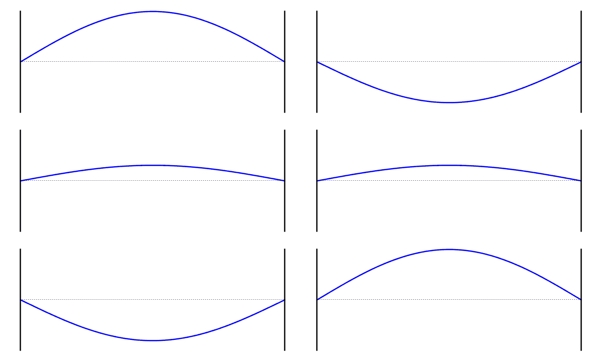
We can explain this a second way using our old friend, the standing wave. At l = 0, the electron is vibrating with a standing wave pattern in all directions around the nucleus, like a guitar string, which vibrates in place instead of vibrating from one end to the other (bridge to tuning pegs, for my guitarists). Visually, this would look like a vibrating sphere, pulsing in and out, up and down, with the waves overlapping where there is the highest likelihood that an electron is there. Since this wave doesn’t “travel” around the nucleus, there can’t be a magnetic field from orbital motion.

So then, what caused the result that Stern and Gerlach saw? We know that they shot a beam of silver atoms through a nonuniform magnetic field. With what we know now, why don’t we take a closer look at silver as an element?
Silver's electron configuration will be the most useful piece of information, which we can find on our trusty periodic table. As we learned in Part 3, the subshells of non-noble gas elements have reactive valence shells. This would be the last parts of the electron configuration, namely the 5s1 orbital.
5, as we know, is the principle quantum number (n). But what do we have here in the orbital quantum number (l) section? An s-orbital! We've just learned s-orbital electrons have no magnetic field due to orbital motion. If that’s the case, wouldn’t the beam of electrons distributed in a line, like our two scientists expected? What gives?
Spin Quantum Number (s)

In the presence of an external magnetic field (B), like the one Stern and Gerlach fired silver atoms through, electrons have two half-spins.
Remember, we don’t believe the electrons actually spin. This is just a representation of the quantum mechanical concept.
Image by William Reusch via Michigan State University
The solution is that the electrons must have some built-in property that gives them some kind of angular momentum. A few years later, in 1925, George Uhlenbeck and Samuel Goudsmit, two Dutch-American scientists, created a term for this built-in angular momentum: spin. For the beam to be split evenly into two, the atoms must have two spins, which they called half-integer spins, +½ and -½. (Note that electrons do not actually spin; this is a term born out of the connection angular momentum has with rotation.)
As a relevant aside, electrons themselves are within a class of subatomic particles known as fermions. Electrons are not the only particles like these. In fact, protons and neutrons are also fermions.
Fermions are opposed by another class of subatomic particle that, as you’d image, has full integer spins (-1, 0, 1, etc.), known as bosons. If we were to plug a boson into the Stern-Gerlach experiment, we would see a third line, corresponding to the spin quantum number of 0, in between the -1 and 1 lines. Fermions and bosons are the two categories in which all particles in the universe reside.

The Higgs Boson
You’ve likely heard of this particle before. It’s one example of how the conception of quantum mechanical ideas often comes far ahead of the experimental proof, just as the idea of quantum mechanics spearheaded by Bohr and Einstein came ahead of the Stern-Gerlach experiment. This boson was discovered in 2012. But when did British theoretical physicist Peter Higgs conceive of this boson? 1964.
- Image of the Higgs Boson
Summary of The Four Quantum Numbers
So…now that we’ve gone through all of the quantum numbers, I think a summary is in order!
The Principle Quantum Number (n) determines the energy level, and thus, the electron’s shell. It is conventionally shown with a number from 1 to 5.
The Orbital Quantum Number (l) determines where the electrons are with respect to the nucleus. It shows the sub-shell and is typically denoted with a letter (s, p, d or f) according to its number (0, 1, 2 and 3).
The Magnetic Quantum Number (m) tells how many subshells there are. It is determined by looking at the subshell and taking the range from -l to l.
Lastly, the complex Spin Quantum Number (s) determines whether the electron’s “spin” is +½ or -½.
Furthermore, all atoms fall under Pauli Exclusion Principle, ensuring that no electrons within an atom have the same quantum mechanical state. It was the aforementioned spin quantum number that proved this; remember that the electrons in the Stern-Gerlach did not simply mix – there was a distinction between +½ and -½. Furthermore, given that the Principle only works with differing quantum mechanical states, only fermions follow this Principle.


Image via futurespaceprogram
This opens up a very important piece of orbital theory.
That spin quantum number shows a great deal, indeed, folks. Because that Pauli Exclusion Principle makes it so that each subshell can only have two electrons – one with the positive spin and one with the negative spin.
And that, my friends, will lead us into the Aufbau Principle, the ending of the first leg of this atomic journey, which we will discuss next time.
This has been quite the undertaking to learn, I understand. Don’t be afraid to ask questions, as scientists do. And share amongst all of your friends – not just the ones interested in science. We can all learn. We just need to light the fire.