
8 - Drawing Molecular Orbital Diagrams

Abstract (TL;DR)
Molecular orbital diagrams are a fantastic way of visualizing how molecular orbitals form using what we already understand about sigma and pi bonds. Depending on if it is a homonuclear case, where the bonding atoms are the same, or a heteronuclear case, where the bonding atoms are different, these molecular orbital diagrams will look incredibly different. Regardless, consideration of the symmetry between atoms, how the orbitals mix and the electronegativities of all atoms are necessary in drawing molecular orbital diagrams. This lesson walks through those considerations.
———
The waves of electrons within atomic orbitals (left and right) forming a pi molecular orbital (top, middle) through destructive interference and a sigma molecular orbital (top, bottom) through constructive interference.
Organization of electrons within molecular orbitals is quite a bit more involved than atomic or hybridized orbitals. In fact, it’s that complexity that makes it so that the simpler valence bond (VB) theory is the preferred way to teach chemical bonding. However, as we discussed, molecular orbital (MO) theory introduces a level of detail missing from valence bond theory.
To make sense of the complexities introduced by antibonding, we build molecular orbital diagrams. These, however, also have their own depth; diagrams like these change according to if you’re working with homonuclear molecules - molecules made of one element - or heteronuclear molecules - molecules made of different elements. Yes, readers, unfortunately, this is going to be similar to the functional groups section in its depth. So let’s start slowly and, first, describe what these diagrams are at their most basic.
Molecular Orbital Diagram
As we’ve established, bonding and antibonding interactions are the key to molecular orbital theory. In fact, the idea of molecular orbitals, the distribution of electrons across a molecule, arises from how electrons distribute themselves energetically.
Remember, antibonding occurs when electrons feel a force that prevents them from engaging in bonding. This would only happen if electrons were distributed in such a way that caused them to destructively interfere with each other. In that case, you might imagine that the energy of the electrons would increase, and, you would be right - as electrons near each other, energy increases (one might call that a very fundamental lesson).
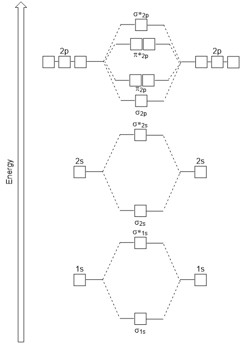
Image by Jessie A. Key via Introductory Chemistry - 1st Canadian Edition (Chapter 9)
Given that some electrons exist in these “antibonding regions” and others exist in the “bonding regions”, we can redefine molecular orbitals as “the distribution of antibonding and bonding electrons across a molecule”.
This, of course, needs to be represented somehow - just like we’ve modeled atomic orbitals and hybridized orbitals. That is where the molecular orbital diagram (MOD) comes in.
At first glance, these diagrams looks terrifying. However, we can rely on a lot of what we already know to help us understand what’s going on here.
Parts of the MOD
First, as we’ve learned, the more electrons that an atom has, the higher its cumulative energy. MODs reflect this by having the lowest atomic orbitals at the bottom of the diagram and the highest orbitals toward the top.
You’ll also notice that each module in a molecular orbital diagram has two sides and a middle section. Each of the two sides represent the atomic orbitals of each atom involved in the bonding, while the middle section represents the molecular orbital formed as the atomic orbitals combine. As you would imagine, the meat (and the complexity) is in the middle of this sandwich.
Check Your Electrons
You can always check if you’ve written your diagrams correctly by adding the atomic orbitals together and seeing if they equal the molecular orbitals. You can also add the number of each orbital type’s electrons; they should also be equal.
Organizing Molecular Orbitals
These diagram reveal just how complementary the MO theory and VB theory are through the presence of the sigma (σ) and pi (π) symbols. In molecular orbital theory, sigma and pi mean the same thing that they meant in valence bond theory, with a few exceptions.
Firstly, we now add our newly acquired antibonding molecular orbitals. There are now four types of orbitals to concern ourselves with: (1) sigma bonding, (2) sigma antibonding, (3) pi bonding, and (4) pi antibonding.
The way these bonds are placed on any molecular orbital diagram is according to how the atomic orbitals that make the MOs mix. In that mixing, there are two factors to consider: (1) atomic symmetry and (2) mixing.
Image via Chegg
Symmetry
As a bond occurs, a bond or internuclear axis - the line that connects the nuclei of two bonded atoms - forms.
Internuclear axes aren’t new to us - they’ve existed ever since we started speaking about bonds. Further, in introducing sigma and pi bonds, we’ve already begun the conversation about symmetry. It is symmetry that defines what sigma and pi mean with respect to molecular orbital theory.

In the diatomic hydrogen molecule to the right, if one were to rotate the two overlapped atomic orbitals about their internuclear axis and no change results — constructively interfering (in-phase) atomic orbitals continued to constructively interfere and vice versa for destructively interfering (out-of-phase) atomic orbitals — you would have an example of sigma bonding or antibonding molecular orbital (according to the phase). We call this symmetry.

Image from Dr. Adam via Professor Adam Teaches
An example of 1s atomic orbitals combining to form: (top) a sigma bonding molecular orbital and (bottom) a sigma antibonding molecular orbital. Take note that, in both, if you rotated the molecular orbital, there are no changes in phase, making them sigma.
Pi molecular orbitals, as you might have already guessed, are the opposite. They form when there is a change in phase after rotating two overlapped atomic orbitals about the internuclear axis. We call this asymmetry.

Image from Dr. Adam via Professor Adam Teaches
An example of the pi antibonding orbital, formed from out-of-phase 2p orbitals. Note how, after rotating, the result is different - a phase change.
| Sigma | Symmetry |
|
|||
| Pi | Asymmetry |
|
|||
In other words, sigma molecular orbitals are the result of symmetric interactions between atomic orbitals, while pi molecular orbitals are the result of asymmetric interactions.

Advanced Symmetries
When we leave the p orbitals and move into the d and f orbitals, we gain not only sigma and pi molecular orbitals, but also delta (δ) and, potentially, phi (φ) molecular orbitals as well.
Mixing
With terms like “overlap” and “combine”, you might be confused as to why I’m singling out “mixing”. Mixing is a little more complex.
“Mixing” is a theoretical explanation for how certain atoms interact to form molecular orbitals. This mixing is similar to hybridizing, wherein atomic orbitals change to stabilize a molecular orbital’s energy distribution. The main difference is that hybridization occurs independently of any other atomic orbitals, while mixing happens between two or, sometimes, more atomic orbitals.
With that said, how does mixing happen? To explain, let’s put two nitrogen atoms together and explain our first type of molecular orbital - homonuclear molecular orbitals.
Homonuclear Molecular Orbitals
Image via Bartleby
Molecular orbital diagram of diatomic nitrogen.
Homonuclear molecular orbitals are formed between two elements that are the same, meaning that they are naturally symmetrical and will perfectly overlap.
However, before we fill out this diagram, compare this MOD to the one above, particularly in the 2p region. They’re pretty similar, except with their sigma and pi bonding molecular orbitals. That’s because diatomic nitrogen exhibits the effects of mixing, which lowers the energy of the sigma 2p MO to below that of the pi 2p MO. But how?
To explain, we have to go back to a classic - effective nuclear charge. The effective charge determines how many reactive electrons can be drawn to an atom. We also know that the effective charge increases as the periodic group increases, or as you go further to the right on the periodic table.
But something happens to the orbitals the higher the effective charge gets - they shrink. Simply put, as electrons are more attracted to the nucleus in atoms with higher effective charges, the sizes of the orbitals become smaller and tighter.
In terms of atomic energy, as orbital sizes decrease, they start to become more uniform - that is, the energies of higher orbitals begin to come closer to the energy of lower ones. Further, the energy of lower orbitals also rises. It is this interaction between orbitals that gives “mixing” its name.
With that said, the specific mixing that occurs in diatomic nitrogen is called sp mixing, which is mixing between the sigma 2s and 2p MOs.
Nitrogen, as we know, has the configuration [He]2s 2 2p 3 . That means that one nitrogen atom has 2 core electrons and 5 valence electrons, for a total of 14 electrons, when factoring both nitrogen atoms - the first display of differences between molecular orbital theory and valence bond theory.
To fill the diagram, first, we fill each side of the diagram with the electrons according to nitrogen’s electron configuration - [He]2s 2 2p 3 . Next, we fill the middle section with the molecular orbital’s electron configuration using Hund’s Rules , just as we do with atomic orbitals. We fill each shell with two electrons before moving to the next, and, for the orbitals with multiple subshells, like the 2p shell, we fill each subshell with one electron before completing the subshell with the second.
The result is:

Image via Bartleby

Limits of sp Mixing
In the second period, only lithium to nitrogen undergo sp mixing, when one is bonded to itself. Oxygen and fluoride do not.
What about diatomic oxygen?
Well, s-p mixing doesn’t occur with diatomic oxygen, creating a molecular orbital diagram like the first in this article. This is because, as more electrons are added to a system, the higher the energy becomes, due to their electrostatic repulsion. If the energy of the 2s and 2p orbitals are too far apart, mixing won’t occur. Therefore, you get a molecular orbital diagram that’s what you expect - the sigma molecular orbital being lower energy than the pi molecular orbital.
With that change in mind, filling this MOD is the same as filling diatomic nitrogen’s:

Note the swapped sigma and pi 2p MOs.
Homonuclear MODs show quite a bit of the ingenuity of this bonding theory because it’s as though it is a natural continuation of the atomic orbitals we know and love. Heteronuclear MODs, on the other hand, are a lot more involved.
Heteronuclear Molecular Orbitals

Carbon Monoxide, composed of a carbon atom (red) and oxygen atom (gray)
Carbon Monoxide. The reason you want to be wary of heating sources, and one of those no-no chemicals when it comes to sustaining human life.
This molecule is interesting. Despite neither carbon or oxygen having stability on their own, from the point of their molecular orbitals, it is a stable molecule. But how is its electrons organized from the perspective of a molecular orbital diagram?
For heteronuclear molecules like these, the first consideration is electronegativity. Electronegativity, if you recall, is the tendency of an atom to pull electrons toward its nucleus. We know that the closer electrons are to the nucleus, the more stable the atom is (the reason that core electrons aren’t reactive).
This means that electronegative atoms have lower atomic energy than electropositive atoms. This results in a MOD that has a “slanted” form.
Carbon monoxide’s MOD, not including the core, nonbonding electrons within each atom’s 1s orbital.
The electronegativity also influences the character of these molecular orbitals. Imagine it this way - oxygen is ravenously drawing all nearby electrons closer. Carbon, as passive as it is, is alright with being dragged along with its electrons. In this situation, which atom influences the shape of the molecular orbitals the most? And in what ways?
Well, since molecular orbitals are composed of both bonding and antibonding orbitals, we can say that oxygen influences the bonding aspect the most since its electronegativity is a constructive force for bonding. Further, if oxygen’s atomic orbitals are influencing the bonding molecular orbitals, then carbon’s atomic orbitals would influence the antibonding molecular orbitals.
This makes the position of the molecular orbitals a little clearer. Can you see how the bonding and antibonding orbitals skew toward either carbon or oxygen?
This demonstrates a valuable rule within MO theory: when atomic orbitals do not have the same energy levels, the molecular orbital that’s formed is most similar to the atomic orbital that is closest to it in energy.
Mixing also occurs between heteronuclear MOs, if the energy between the atoms is close enough. This is the case in carbon monoxide, in which sp mixing occurs.
Sp mixing is a bit different in heteronuclear MOs, but the concept is the same. Molecular orbitals that are close enough in energy will mix, but, due to the differences in electronegativity, the symmetries of each atom’s orbitals become more important. Fortunately, our molecular orbital diagram above uses dotted lines to demonstrate which atomic orbitals mix to form which molecular orbitals.
Even more fortunate is, once you’ve determined how to draw the molecular orbital diagram, the rules for filling MO diagrams remain the same as always. Our filled MO is:

Loose Ends
If you made it through that explanation of molecular orbital theory, you’ve learned something that even college students struggle with - very well done. But, going through it, you might have some questions.
First, the d orbital. Since it’s got 5 subshells, there’s a lot less likelihood that there is symmetry between them. That means, there are only a few combinations of atomic orbitals that may work to form molecular orbitals. That is also why educators prefer to teach MO theory using the elements in the first and second period - the s and p orbital elements.
But, perhaps more importantly, in the last lesson, I referenced that the idea of valence bond theory being insufficient, as the idea of electrons being solely located in between atoms is unrealistic. These systems, also known as localized systems, make understanding bonding very simple (hence why bonding is taught with the valence bond theory). However, we needed molecular orbital theory - a delocalized system, where electrons are distributed all throughout a molecule instead of just one area - to explain the more realistic scenario. This lack of an explanation for delocalization was one of the biggest weaknesses of valence bond theory.
However, my mentioning of its weakness doesn’t mean that valence bond theory doesn’t have an answer at all. With our understanding of delocalized systems in the molecular orbital theory, we’ll discuss delocalization within the valence bond theory in the next lesson.